Chapter 4: Group Relative Policy Optimization (GRPO) and beyond

Preface

This article marks Chapter 4 — the final installment in our Reinforcement Learning for LLMs series. If you’ve been following along, we’ve journeyed from the foundations of RLHF to advanced optimization methods, laying the groundwork for understanding how reinforcement learning shapes large language models.

For new readers, we recommend exploring the earlier chapters first to build context:

• Chapter 1: What is Reinforcement Learning
• Chapter 2: Value based Reinforcement Learning and policy based reinforcement learning
• Chapter 3: Actor Critic methods, PPO.

In this concluding chapter, we explore Group Relative Policy Optimization (GRPO) and its successors — DAPO and GSPO — to understand how these methods advance the state of RL-based fine-tuning for LLMs in terms of efficiency, scalability, and stability

Introduction

Welcome back to the final chapter of our Reinforcement learning series! We hope that you have thoroughly enjoyed our content so far and you’ve learned a lot about modern reinforcement learning algorithms and how to implement them. In the previous chapter, we explored actor-critic methods which marry both a value-based function and an actor which follows a causal probabilistic distribution.

In this chapter, we will explore the more modern methods which are associated with the field of Reinforcement learning applied / tailored specifically for Large Language Models (LLMs), starting with Group relative policy optimization (GRPO).

By the end of this chapter, our hope is that you are familiar with all the modern reinforcement learning techniques that are currently applied for LLM post-training and can start training your models leveraging these methods using your dataset of your choice!

Alright, so without any further ado, let’s commence!

Recap: Proximal Policy Optimisation

Proximal Policy Optimisation is an actor-critic method which maintains two components:

• The actor is the policy $\pi_\theta$ - it decides what action to take in a given state (e.g., what token to generate).
• The critic is a learned value function - it estimates how good an actor or state is, guiding the actor’s learning through advantage estimates.

The Final PPO Objective Function

$$L_{\text{total}}(\theta) = L_{\text{CLIP}}(\theta) - c_1 L_{\text{VF}}(\phi) + c_2 H[\pi_{\theta}]$$

Where,

1. The Clipped Surrogate Objective ($L_{\text{CLIP}}$): Our policy improvement signal

2. The Value Function Loss ($L_{\text{VF}}$): Trains the critic to better estimate state values $L_{\text{VF}}(\phi) = \mathbb{E}_t \left[ \big(V_\phi(s_t) - V_t^{\text{target}}\big)^2 \right]$

3. The Entropy Bonus ($H[\pi_{\theta}]$): Encourages exploration by rewarding policy uncertainty \( H[\pi_{\theta}] = \mathbb{E}_t\left[-\log \pi_\theta(a_t \mid s_t)\right] \)

The coefficients $c_1$ and $c_2$ balance the relative importance of value learning and exploration against the main policy objective.

If the equation above feels daunting to you, we urge you to read part 3 of our series before proceeding further.

The Bottleneck

Often, the value function employed in PPO is another neural network which is comparable in size as the policy model, it brings a substantial memory and computational burden - which make it notoriously compute intensive to optimize the model. And furthermore, in practice, there is a per-token KL penalty from a reference model (in most cases, it is simply the frozen copy of the policy model) applied in the reward at each token viz.,

$r_t = r_\phi(q, o_{\leq t}) - \beta \log \frac{\pi_\theta(o_t \mid q, o_{<t})}{\pi_{\text{ref}}(o_t \mid q, o_{<t})}$

Where,

• $r_\phi$ : Reward model
• $\pi_{\text{ref}}$ : Reference model, which is usually the initial Supervised finetuned model and,
• $\beta$ : KL penalty

In LLM reinforcement learning, the rewards are disbursed at the end of a sequence completion (i.e., at the very last token), and therefore, might serve to complicate the training of a value function that is accurate at each token.

The Addressal

The authors of the seminal GRPO (Group Relative Policy Optimization) paper posited this question, “What if we didn’t need a critic at all?”

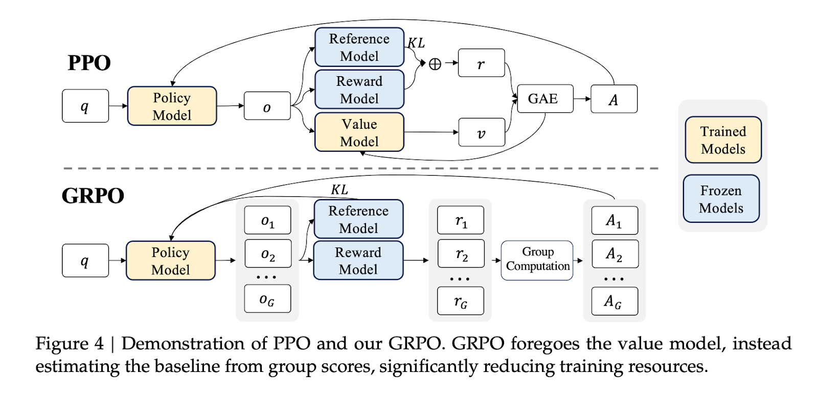
GRPO avoids the computational overhead posed by Proximal Policy Optimization (PPO) by obviating the need for an additional value function approximation as seen in PPO, and instead uses the average normalised reward of multiple sampled outputs (the “G” in GRPO) a policy model produces in response to the same question, as the baseline. More specifically.

1. Sample $G$ responses \(
   o_i, \; i=1,\dots,G \sim \pi_{\theta_{\text{old}}} \text{ for each prompt } q
   \)
2. Use a reward model to assign ${r_1, r_2, ..., r_G}$
3. Compute normalised advantages:

$$ \hat{A}_{i,t} = \frac{r_i - \text{mean}(r)}{\text{std}(r)} $$

4. Optimise the GRPO objective:
   
   \[
   \begin{aligned}
   J_{GRPO}(\theta) &= \mathbb{E}_{q \sim P(Q), o_i \sim \pi_{\theta_{old}}} \Bigg[ \\
   &\quad \frac{1}{G} \sum_{i=1}^{G} \frac{1}{|o_i|} \sum_{t=1}^{|o_i|}
   \min \Bigg(
   \frac{\pi_\theta(o_{i,t} \mid q, o_{i,<t})}{\pi_{\theta_{old}}(o_{i,t} \mid q, o_{i,<t})} \hat{A}_{i,t},
   \text{clip}(\cdots)
   \Bigg) \\
   &\quad - \beta D_{KL}(\pi_\theta \,||\, \pi_{ref}) \Bigg]
   \end{aligned}
   \]

This might look slightly terrifying, but let’s look at the core of this objective:

\(
\min \left(
\frac{\pi_\theta(o_{i,t} \mid q, o_{i,<t})}{\pi_{\theta_{old}}(o_{i,t} \mid q, o_{i,<t})} \hat{A}_{i,t},
\text{clip}(\cdots)
\right)
\)

Which is exactly the PPO objective we covered in the previous chapter! Just stretched across multiple completions $o_i$. So the key innovation in GRPO can be summarised as the following:

Instead of a critic-based $\hat{A}_{i,t}$, GRPO uses a group-normalised advantage. That is, it rewards samples that are better than their siblings, and penalises the worse ones, without needing a separate value function at all. The last part is critical, as it helps us bypass a lot of computational overhead that was introduced by PPO.

Understanding Importance Sampling: Some Tidbits On Which Many Redressals Of GRPO Are Based Upon

Before we examine how GRPO's refinements address specific failure modes, we need to understand the mathematical machinery underlying all these algorithms: importance sampling. This isn't just a technical detail - it's the reason these methods work at all, and understanding where it breaks down is key to appreciating why DAPO and GSPO exist.

The Core Problem

Suppose we want to compute the expected value of some function $f(x)$ under a target distribution $p_{\text{target}}(x)$:
\(
\mathbb{E}_{x \sim p_{\text{target}}}[f(x)] = \int f(x)\, p_{\text{target}}(x)\, dx
\)

In reinforcement learning, this expectation might represent the expected reward under our new, updated policy. The straightforward approach would be to sample many trajectories from $p_{\text{target}}$, evaluate $f$ on each, and average the results.

But here's the problem: sampling is expensive. Generating even a single completion from a 70B parameter language model can take seconds. Generating thousands of completions after every gradient update would make training prohibitively slow.

The Importance Sampling Solution

Importance sampling offers an elegant workaround. Suppose we already have samples from a different distribution $p_{\text{behavior}}(x)$ - say, from our policy before the most recent update. Can we reuse those samples to estimate the expectation under $p_{\text{target}}$?

Yes, we can, through a simple mathematical trick. We rewrite our target expectation as:

\(
\mathbb{E}_{x \sim p_{\text{target}}}[f(x)] = \int f(x)\, p_{\text{target}}(x)\, dx
\)

Multiply and divide by $p_{\text{behavior}}(x)$:

\(
\mathbb{E}_{x \sim p_{\text{target}}}[f(x)] = \int f(x)\, \frac{p_{\text{target}}(x)}{p_{\text{behavior}}(x)} \, p_{\text{behavior}}(x)\, dx
\)

which gives:

\(
\mathbb{E}_{x \sim p_{\text{target}}}[f(x)] = \mathbb{E}_{x \sim p_{\text{behavior}}}\left[ \frac{p_{\text{target}}(x)}{p_{\text{behavior}}(x)} f(x) \right]
\)

This is the importance sampling identity. It tells us we can estimate expectations under $p_{\text{target}}$ using samples from $p_{\text{behavior}}$, as long as we weight each sample by the importance ratio:

\(
w(x) = \frac{p_{\text{target}}(x)}{p_{\text{behavior}}(x)}
\)

In practice, if we have $N$ samples ${x_1, x_2, \ldots, x_N}$ drawn from $p_{\text{behavior}}$, our estimate becomes:

\(
\mathbb{E}_{x \sim p_{\text{target}}}[f(x)] \approx \frac{1}{N} \sum_{i=1}^{N} w(x_i) f(x_i)
\)

Application to Policy Gradient RL

In reinforcement learning:

• Target distribution: the new policy $\pi_\theta$ (after an update)
• Behavior distribution: the old policy $\pi_{\theta_{\text{old}}}$ (which generated our rollout data)
• Function of interest: the advantage-weighted log probability, which drives policy improvement

For a single token $o_t$ generated in context $(q, o_{<t})$, the importance ratio is:

$$
w_t = \frac{\pi_\theta(o_t \mid q, o_{<t})}{\pi_{\theta_{\text{old}}}(o_t \mid q, o_{<t})}
$$

This ratio tells us how much more (or less) likely the new policy is to generate this token compared to the old policy.

• If $w_t > 1$, the new policy favours this token more.

If $w_t < 1$, it favours it less.

When Importance Sampling Breaks Down

Importance sampling only works well when $p_{\text{target}}$ and $p_{\text{behavior}}$ are reasonably similar. If they diverge too much, the importance ratios become extremely variable - some very large, some very small - leading to high-variance estimates.

The variance of the importance sampling estimator is:

$$
\text{Var}\left[\frac{p_{\text{target}}(x)}{p_{\text{behavior}}(x)} f(x)\right]
$$

If $p_{\text{target}}$ assigns high probability to regions where $p_{\text{behavior}}$ assigns low probability, the ratio $\frac{p_{\text{target}}(x)}{p_{\text{behavior}}(x)}$ can explode. A single sample with an enormous weight can dominate the entire estimate, making training unstable.

This is why clipping exists. In PPO and GRPO, we constrain importance ratios to the range $[1 - \epsilon, 1 + \epsilon]$, preventing any single token from having an outsized influence:

$$
\min\left(w_t A_t, , \text{clip}(w_t, 1 - \epsilon, 1 + \epsilon) A_t\right)
$$

This says: we trust importance sampling corrections up to a point, but beyond that, we’d rather be conservative than risk instability.

The Token-Level Problem in GRPO

Here’s where GRPO’s design becomes problematic.

Importance sampling theory requires multiple samples from the behavior distribution to effectively correct for distributional mismatch. The law of large numbers ensures that, averaged over many samples, the weighted estimator converges to the true expectation.

But GRPO applies importance weights at the token level, where each token comes from a single trajectory. We’re not averaging multiple samples of “what’s the next token given this context?” — we only have one sample: the token that was actually generated.

This violates the conditions under which importance sampling provides reliable estimates. Instead of correcting for distribution shift, these per-token ratios introduce high-variance noise, especially in long sequences where this noise compounds multiplicatively.

For a sequence of length $T$, the cumulative effect of noisy token-level ratios is:

$$
\prod_{t=1}^{T} w_t = \prod_{t=1}^{T} \frac{\pi_\theta(o_t \mid q, o_{<t})}{\pi_{\theta_{\text{old}}}(o_t \mid q, o_{<t})}
$$

Even if individual ratios are only slightly noisy, their product can vary wildly, making the gradient estimate unreliable. This is especially catastrophic in Mixture-of-Experts architectures, where even small policy changes can activate entirely different experts per token, causing large ratio fluctuations for structural, not semantic, reasons.

Beyond GRPO: Stability, scale and theoretical refinements

GRPO has become a very popular choice for LLM post-training. But with any algorithm deployed at scale, there were some emergent challenges. Since the release of the paper, the research community has put forth a lot of modifications on how to improve various aspects of this algorithm.

The section that follows isn’t a tournament to proclaim the best algorithm, but merely a brief examination of two notable refinements on GRPO: DAPO (Dynamic Advantage Policy Optimization) and GSPO (Group Sequence Policy Optimization). Let’s talk about them quickly

DAPO: Stability, And Lower Variance At Scale

While GRPO elegantly sidesteps the critic, it inherits a subtle vulnerability: the assumption that sampling alone guarantees useful learning signals. In practice, this breaks down. DAPO addresses four specific failure modes that emerge during large-scale training:

The Problem: When Gradients Go Silent (or Noisy)

Consider a typical GRPO training step. You sample a group of $G$ outputs, score them using a reward function (e.g., exact match or answer relevance), and compute normalised advantages within the group:

$$ \hat{A}_{i,t} = \frac{r_i - \text{mean}(r)}{\text{std}(r)} $$

But what happens when:

• All responses are correct? Advantage becomes zero. No learning signal.
• All responses are wrong? Same outcome. No gradient.

The Solution Proposed By DAPO’s Authors:

DAPO introduces four design choices, each addressing a specific instability:

1. Decoupled Clipping ("Clip-Higher")
   The authors observed a subtle but critical problem with symmetric clipping: it creates a "Matthew Effect" where tokens that the old policy already favored continue to be reinforced, whilst promising low-probability tokens get clipped away before they can improve. Consider a concrete example: suppose the old policy assigned probability 0.2 to a crucial token (it barely sampled it), but this token has positive advantage (it's actually good!). With $\epsilon = 0.2$, the upper bound becomes $0.2 \times 1.2 = 0.24$. Even if the current policy recognizes this token's value and raises its probability to 0.4 - a 2× improvement - it gets clipped! The gradient becomes zero, and the model never learns to favor this token. Contrast this with a token the old policy already favored at probability 0.9. The upper bound is $0.9 \times 1.2 = 1.08$, which exceeds the maximum probability of 1.0, so it's never clipped. DAPO's solution: use separate bounds $\epsilon_{\text{low}}$ and $\epsilon_{\text{high}}$, giving more breathing room ($\epsilon_{\text{high}}$ can be 2-3× larger) for increasing probabilities of promising low-probability tokens, whilst still constraining decreases. This asymmetry keeps exploration alive

2. Dynamic Sampling

Rather than accepting batches where all samples share the same label (all correct or all incorrect), DAPO re-samples until the group contains contrast - at least one correct and one incorrect output. This structural constraint ensures gradients always have meaningful signals.

3. Token-level averaging

GRPO's averaging structure creates an attribution problem that becomes severe with variable-length responses. Consider sampling two responses: one with 200 tokens, another with 10 tokens. In GRPO's formula $\frac{1}{G} \sum_{i=1}^{G} \frac{1}{|o_i|} \sum_{t=1}^{|o_i|}$: - Each token in the 200-token response contributes: $(1/200) \times (1/2) = 1/400$ - Each token in the 10-token response contributes: $(1/10) \times (1/2) = 1/20$ The shorter response's tokens have 20× more influence on the gradient, despite both responses answering the same question. For complex reasoning tasks requiring lengthy explanations, this severely dilutes the learning signal. DAPO's solution: $\frac{1}{\sum_{i=1}^{G} |o_i|} \sum_{i=1}^{G} \sum_{t=1}^{|o_i|}$ treats all 210 tokens equally, each contributing $1/210$ to the final gradient. Longer, high-quality responses now properly influence training

4. Overlong Reward Shaping

Standard practice assigns a uniform punitive reward to truncated samples (those exceeding the maximum sequence length). However, this introduces noise: a valid reasoning process may be penalised purely for its length, potentially confusing the model about the quality of its reasoning. DAPO introduces a length-aware penalty mechanism that operates within a tolerance interval. Rather than punishing all truncated samples equally, longer responses within this interval receive progressively stronger penalties, whilst shorter responses near the threshold are treated more leniently. This soft punishment approach signals the model to avoid excessive verbosity without discarding potentially sound reasoning that happens to be lengthy. The result is a reward signal that better reflects real-world preferences: responses should be concise, but not at the expense of completeness.

The Final DAPO Objective

\(
J_{\text{DAPO}}(\theta) = \mathbb{E}_{o_i, i=1,\dots,G \sim \pi_{\text{old}}} \Bigg[
\frac{1}{\sum_{i=1}^{G} |o_i|} \sum_{i=1}^{G} \sum_{t=1}^{|o_i|}
\min\Big(
r_{i,t}(\theta) \hat{A}_{i,t},
\operatorname{clip}(r_{i,t}(\theta), 1 - \epsilon_{\text{low}}, 1 + \epsilon_{\text{high}}) \hat{A}_{i,t}
\Big)
\Bigg]
\)

subject to:

\(
0 < \left| \{ o_i \mid \text{is\_equivalent}(a, o_i) = \text{True} \} \right| < G
\)

This, as you can see, follows the same structure that we’re familiar with:

• The $\min(\cdot, \text{clip}(\cdot))$ is our PPO core
• The $r_{i,t}(\theta)$ ratio is still the trust score: how much more confident the new policy is about a token, compared to the old one - same as GRPO
• And $\hat{A}_{i,t}$? It is the advantage - group-normalised just like GRPO

The key structural change lies in how we aggregate and normalize. GRPO computes $\frac{1}{G} \sum_{i=1}^{G} \frac{1}{|o_i|} \sum_{t=1}^{|o_i|}$ - averaging within each sequence first (dividing by $|o_i|$), then averaging across sequences (dividing by $G$). This gives each sequence equal weight. DAPO instead uses $\frac{1}{\sum_{i=1}^{G} |o_i|} \sum_{i=1}^{G} \sum_{t=1}^{|o_i|}$—summing all tokens across all sequences, then normalizing by the total token count. This gives each token equal weight, meaning longer sequences contribute proportionally more to the gradient. This structural change is what enables the token-level loss attribution we discussed - individual token quality now matters independently of sequence-level outcomes.

In essence, DAPO isn’t a reinvention of GRPO - it is merely meant to be its more stable counterpart over longer training horizons.

GSPO: A Better Theoretical Foundation

Whilst DAPO was intended to address practical training issues arising from GRPO, GSPO (Group Sequence Policy Optimization) tackles something more fundamental: a mathematical inconsistency at the heart of GRPO’s design.

The Problem with GRPO: A Unit Mismatch

GRPO (Group Relative Policy Optimisation) compares multiple responses to the same query and estimates advantages based on normalised group rewards. But the actual optimisation it performs is at the token level:

$w_{i,t}(\theta) = \frac{\pi_{\theta}(y_{i,t}|x, y_{i,<t})}{\pi_{\theta_{\text{old}}}(y_{i,t}|x, y_{i,<t})}$

Each token’s gradient is scaled by this ratio, despite the fact that the reward $r(x, y_i)$ is only ever assigned to the entire sequence $y_i$.

The principle of importance sampling is to estimate the expectation of a function under a target distribution $\pi_{tar}$ by re-weighting samples drawn from the current or behaviour distribution $\pi_{beh}$ - this is reliant on averaging multiple samples from the behaviour distribution to effectively correct for distributional mismatch. In contrast, GRPO applies importance weight  $\frac{\pi_{\theta}(y_{i,t}|x, y_{i,<t})}{\pi_{\theta_{\text{old}}}(y_{i,t}|x, y_{i,<t})}$ tokens drawn from a single sample - this leads to importance sampling not doing its intended role. Additionally, this misalignment introduces two headaches:

• High-variance gradients: Since these token-level ratios are computed from single samples of the next-token distribution, they're noisy.
• Sequence-length compounding: That noise stacks up at every step

For Mixture-of-Experts (MoE) models, where different experts activate for different tokens, this becomes catastrophic. GRPO attempts to mitigate this with "routing replay" (caching and freezing expert paths), but that's a brittle workaround

The Solution: Sequence-Level Optimization

GSPO makes a simple but profound change: if rewards live at the sequence level, the optimisation should too. Instead of per-token ratios, GSPO defines a sequence-level importance ratio as the geometric mean of token-level ratios:

$s_i(\theta) = \left( \prod_{t=1}^{|y_i|} w_{i,t}(\theta) \right)^{1 / |y_i|} = \left( \frac{\pi_{\theta}(y_i|x)}{\pi_{\theta_{\text{old}}}(y_i|x)} \right)^{1/|y_i|}$

‍

Where $w_{i,t}(\theta)$ are the same token-level ratios as observed in GRPO. The difference here is that in GSPO, these are computed as building blocks, which are then collapsed into a single scalar $s_{i}(theta)$ that is applied uniformly across the entire sequence. In GRPO, each token receives its own individual importance weight; in GSPO, all tokens in sequence $i$ share the same sequence-level weight.

Why geometric mean? Well, because it naturally dampens the extremes:

• A single volatile token doesn’t wreck the entire ratio.
• Extremely low-likelihood tokens correctly suppress the whole sequence - matching the intent of the reward.
• More numerically stable than the arithmetic mean.

Final GSPO Objective

GSPO defines the RL objective as:

$J_{\text{GSPO}}(\theta) = \mathbb{E}_{{x, y_i} \sim \pi_{\text{old}}} \left[ \frac{1}{G} \sum_{i=1}^{G} \min\left(s_i(\theta) \hat{A}_{i}, \operatorname{clip}(s_i(\theta), 1 - \epsilon, 1 + \epsilon) \hat{A}_{i}\right) \right]$

Where the advantage is computed using group-normalised rewards:

$\hat{A}_i = \frac{r(x, y_i) - \text{mean}(r)}{\text{std}(r)}$

This is almost poetically symmetric: each sequence's gradient gets scaled based on how much better it did than its siblings (responses to the same prompt), modulated by how off-policy it is (via $s_i(\theta)$).

And just like before, this objective is not too dissimilar from what we’ve covered so far. And I am sure you, by now, have got the eye for it. But for the sake of completeness, let’s talk about what’s different in this objective.

• $s_i(\theta)$ is a sequence-level importance weight. It’s the geometric mean of token-level ratios
• $\hat{A}_i$ is a sequence-level advantage, just like in GRPO. The only difference is that it’s at a sequence level. This tells us how good this sequence was compared to its siblings in the group.

Comparative Summary

The evolution from GRPO to its refinements reflects the iterative nature of algorithm development in modern machine learning. Each method optimises for different priorities based on observed failure modes in practice:

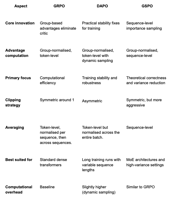
None of these algorithms is universally "better" - they optimize for different constraints and failure modes. DAPO prioritises practical training stability, GSPO prioritises mathematical correctness, and GRPO prioritises simplicity and computational efficiency. Your choice depends on your specific architecture, dataset characteristics, training infrastructure, and the particular pathologies you observe during training.

Closing Thoughts

The trajectory from PPO to GRPO, and subsequently to DAPO and GSPO, reflects a progressive refinement in how reinforcement learning is applied to large language models. Each method builds upon the limitations of its predecessor, first addressing the computational burden of maintaining a critic, then stabilising training dynamics at scale, and finally correcting statistical mismatches in the optimisation objective.

Understanding these algorithms through their mathematical formulation and design motivations reveals the inherent trade-offs in balancing sample efficiency, variance control, and architectural scalability. As models continue to scale and diversify in deployment contexts, from dense transformers to sparse MoE architectures, from short-form dialogue to long-form reasoning, these reinforcement learning techniques provide a robust foundation for aligning policy updates with meaningful behavioural improvements.

The field of LLM post-training via reinforcement learning remains remarkably active. New variants and refinements emerge frequently, each addressing specific pain points observed in production systems. What we've covered here - Starting from what exactly is Reinforcement learning, its different flavours and then leaning more towards LLM Reinforcement learning with PPO, GRPO, DAPO, and GSPO - represents the current state of the art, but certainly not the final word. We can expect further innovations in how we optimize these systems.

Our hope is that this series has equipped you with both the theoretical understanding and practical intuition to implement these methods yourself. Whether you're fine-tuning a model for domain-specific reasoning, aligning outputs to human preferences, or simply experimenting with post-training techniques on your own datasets, you now have the foundational knowledge to make informed choices about which algorithm suits your needs - and more importantly, why.

The mathematics might seem daunting at first, but as you've seen throughout this series, these algorithms all share a common lineage. They're variations on a theme: how do we improve a policy by learning from its own samples, whilst keeping updates stable and well-behaved? Once you internalize that core principle, the rest becomes a matter of understanding the specific tricks each method employs to achieve that goal.

So, what's next?

Well, it's your turn to play! Grab a dataset, pick an algorithm, and start training. There's no substitute for hands-on experience when it comes to understanding the nuances of these methods. You'll encounter gradient explosions, reward hacking, and all manner of training instabilities - and that's exactly how you'll develop the intuition to debug and improve these systems.

The future of LLM alignment is being written right now, and you're equipped to be part of that conversation.

Thank you for following this series! We hope that it has helped you.

Until next time.