Chapter 2: Value Based Reinforcement Learning vs Policy Based Reinforcement Learning

Reinforcement Learning for LLMs in 2025: A Mathematical and Practical Series

Chapter 2: Value-Based vs Policy-Based Reinforcement Learning

Introduction

Welcome back! If you’re just joining us, we recommend starting with Chapter 1: Reinforcement Learning for LLMs in 2025 — A Mathematical and Practical Series, where we explored the core concepts of reinforcement learning (RL) through the lens of Minesweeper - what it is, why it matters, and how it powers the reasoning capabilities of today's Large Language Models (LLMs). We looked at intuitive examples, broke down the vocabulary, and hinted at the rich algorithmic landscape that underpins modern AI systems.

In this chapter, we're turning the page to one of the most fundamental splits in the RL universe: value-based vs policy-based methods.

Why does this split matter? Because it represents two different strategies for learning from the world:

• Should I learn how valuable each move is - and act accordingly? (value-based)
• Or should I directly learn what moves to make, and trust my strategy to evolve? (policy-based)

Continuing our minesweeper analogy from Chapter 1: when you see a "3" tile surrounded by flags, do you first calculate "clicking here gives me a 90% chance of success" (value-based thinking), or do you just instinctively know "I should click here" (policy-based thinking)?

This philosophical divide shapes everything from how agents explore to how they scale with complexity. And, as you'll soon see, it has major implications for how we train LLMs.

Let's break it down.

Recap: What Is the Agent Trying to Do?

Before diving into the two schools of thought, let’s remind ourselves of the big picture.

The goal of an RL agent is simple:

Learn a policy that maximises the expected cumulative reward over time.

In Minesweeper, this means learning a strategy that helps you clear the most mines while avoiding explosions. A policy, to recap, is simply the agent's strategy - a mapping from board states to tile-clicking decisions, or more generally, from state to actions. Given a current board configuration, the policy tells you which tile to click next. It can be either deterministic (always clicks a particular tile in a given configuration) or stochastic (assigns probabilities to different tile choices).

This means:

• Observing the current board state
• Choosing which tile to click
• Receiving feedback (+1 for safe, -10 for mine)
• Improving your clicking strategy over time

But how the agent learns that clicking strategy - that's where the split begins.

Value-Based Methods: Learn to Judge First, Then Act

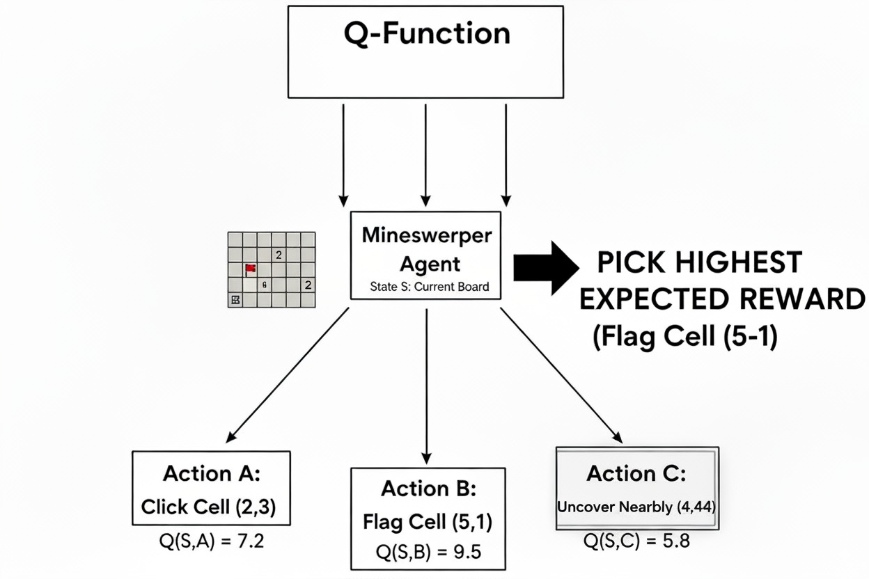
In value-based methods, our Minesweeper player starts by learning a value function - a way to estimate the expected cumulative reward for each possible click.

Instead of directly learning which tiles to click, the player first builds a judgment system that tells them: "If I click on tile (x,y) when the board looks like this, how much reward can I expect in the long run?"

This judgment is encoded as a function: 

$$Q(s, a) = \text{Expected return from taking action } a \text{ in state } s$$

In our Minesweeper context:

• s = current board configuration (which tiles are revealed, flagged, etc.)
• a = clicking on a specific tile (x,y)
• Q(s,a) = expected score from clicking that tile in that board state

Once our Minesweeper player has these Q-values for every possible click, they can act greedily - always pick the tile with the highest expected return.

Q-Learning: The Canonical Value-Based Algorithm

Let's see how this works in practice with our Minesweeper example.

Imagine you're looking at a board where you see a "1" tile with only one adjacent unrevealed square. This is actually one of the safest possible moves in Minesweeper - since the "1" indicates exactly one mine in the surrounding area, and that mine must already be accounted for by other revealed information, this unrevealed square is guaranteed to be safe. Your Q-learning Minesweeper player would:

1. Look at the current state: Board configuration with the "1" and adjacent unrevealed tile
2. Evaluate the action: Calculate Q(current_board, click_adjacent_tile)
3. Take action: Click the tile (it's probably safe since the "1" needs only one mine)
4. Observe outcome: +1 reward (safe click) and new board state
5. Update Q-value: Adjust our estimate based on what actually happened

The Q-learning update rule looks like this: 

$$Q(s,a) \leftarrow Q(s,a) + \alpha[r + \gamma \max_{a'} Q(s',a') - Q(s,a)]$$

Breaking this down in Minesweeper terms:

• Q(s,a): Our current estimate of clicking tile 'a' in board state 's'
• α: Learning rate (how much we adjust our estimate)
• r: Immediate reward (+1 for safe click, -10 for mine)
• γ: Discount factor (how much we care about future rewards)
• s’: The new board state after clicking tile “a” (more tiles revealed, updated information)
• a’: Any possible tile we can click in the new board state s’.
• max Q(s',a'): Best possible move from the new board state
• The whole bracket: Prediction error - how wrong we were

This follows the standard Q-learning algorithm (see the canonical formulation) where we update our current Q-value by learning from the immediate reward plus the discounted value of the best future action 

Why Value-Based Methods Matter

Q-learning and other value-based methods are:

• Sample efficient: This means they can learn from fewer data points by reusing past experiences multiple times. In Minesweeper terms, imagine you store every click you've ever made along with the outcomes - that's your "replay buffer." Even that disastrous game from yesterday where you hit a mine on the second click? You can replay that experience over and over to reinforce "don't click there when the board looks like this." Unlike methods that throw away each game after learning from it once, Q-learning can revisit old games hundreds of times, squeezing maximum learning value from every click you've ever made.
• Good for discrete problems: Perfect for Minesweeper's grid-based tile clicking

But they also struggle with:

• High-dimensional action spaces: Imagine Minesweeper with a million tiles - evaluating every possible click becomes impossible
• Planning over multiple steps: They tend to act greedily, focusing on the next click rather than long-term board strategy

A Note on What "Off-Policy" Means

In our Minesweeper analogy, "off-policy" means you can learn from watching anyone play - even a complete beginner making random clicks.

You can gather experience from different players, store all their games, and reuse them to improve your own Q-values. This is powerful because bad games still teach you which moves to avoid!

Strengths:

• Learns to evaluate moves first, then acts based on best evaluation
• Sample-efficient, off-policy learning leads to quicker convergence
• Can learn from any data, even random play

Weaknesses:

• Doesn't perform well when action space is huge (imagine Minesweeper with millions of tiles)
• Off-policy nature makes it difficult to incorporate prior knowledge about good Minesweeper strategies

Policy-Based Methods: Learn to Act Directly

Policy-based methods skip the value estimation step entirely. Instead of learning "how good is each tile to click" (estimating Q-values), they directly learn "which tile should I click right now?

Going back to our Minesweeper example: instead of calculating expected rewards for every possible tile, our player develops direct intuition about clicking patterns. See a "1" with one adjacent unrevealed tile? Click it immediately. See a corner with a "1" already satisfied? Skip it.

Formally, they parameterise a policy: 

$$\pi_\theta(a \mid s)$$

This is a probability distribution over actions, given state $s$. The parameters $\theta$ are learned via gradient ascent - pushing the policy to favour actions that lead to high reward.

‍

What Does That Mean?

Let's continue our Minesweeper analogy. A value-based learner might analyze thousands of board positions to learn which tile configurations are advantageous, then act accordingly.

But a policy-based learner? It learns to click.

It builds intuition for which tiles to click in which situations, and updates that clicking intuition directly based on game performance.

The Policy Gradient Objective

We define the objective as:

$J(\theta) = \mathbb{E}_{\tau \sim \pi_\theta} \left[ R(\tau) \right]$

Where:

• $\tau \sim \pi_\theta$: A trajectory τ is a sequence of states and actions sampled from the current policy. In minesweeper terms, a complete game trajectory (sequence of tile-clicks) played according to our current strategy.
• $R(\tau)$: The total reward along that trajectory. In minesweeper terms, the total score from that game (safe clicks minus the mine explosions).
  

We update $\theta$ using gradient ascent:

$\theta \leftarrow \theta + \alpha \nabla_\theta J(\theta)$

Where:

• $\alpha$: Learning rate (how big a step we take)
• $\nabla_\theta J(\theta)$: Gradient of expected return w.r.t. the policy parameters

This is the basic idea of policy gradients: increase the probability of actions that lead to high rewards, decrease it for those that don’t. It looks like a clean, elegant idea, however in practice it’s a little too blunt.

Why Basic Policy Gradients Are Too Blunt

Imagine you play two Minesweeper games:

• Game 1: Score +15 (cleared most of the board)
• Game 2: Score -8 (hit a mine early)

Basic policy gradients would say: "Make all moves from Game 1 more likely, make all moves from Game 2 less likely."

But this is too simplistic! Maybe that early risky click in Game 2 was actually brilliant - it just unlocked an unlucky mine. And maybe some "safe" clicks in Game 1 were actually poor choices that got lucky.

This is where the concept of "advantage" comes into play.

Introducing the Advantage

The advantage tells our Minesweeper player: "Was this specific tile click better or worse than my usual clicking performance in similar board situations?"

Let's say you typically score +3 points when you encounter a board configuration with a "2" tile and two adjacent unrevealed squares. Now you're in that exact situation again:

• If clicking the left tile leads to +7 total points: Advantage = +4 (much better than usual!)
• If clicking the right tile leads to +1 total points: Advantage = -2 (worse than your typical performance)

The advantage captures the relative merit of each click, rather than just the absolute game score.

• If the click was better than usual → push the policy more toward that clicking pattern
• If it was worse than usual → tone down that clicking tendency

This concept is baked into the most widely used update rule in modern policy methods:

$\nabla_\theta J(\theta) = \mathbb{E}_t\left[ \nabla_\theta \log \pi_\theta(a_t \mid s_t) \hat{A}_t \right]$ 

I know it might look scary, but don’t worry. Let’s break it down:

• $\pi_\theta(a_t \mid s_t)$: This is the probability of taking action $a_t$ in state $s_t$, under our current policy.
• $\log \pi$: We take the logarithm of that probability (don’t worry why yet - we’ll explain in detail in the next chapter).
•  $\nabla_\theta$: We’re computing the gradient with respect to the policy parameters $\theta$, i.e., nudging them to increase/decrease the probability of actions based on how good they were.
• $\hat{A}_t$: This is the advantage estimate - our feedback signal.
  

This single formulation gives us a powerful way to say: “Let’s move our policy in the direction of better-than-average actions, and avoid the worse ones.”

And that’s why almost every modern RL algorithm - especially those used to train LLMs - relies on advantage-based policy updates.

We'll build more formal intuition for this in the coming chapters. For now, just keep in mind: advantage ≠ reward, it's better.

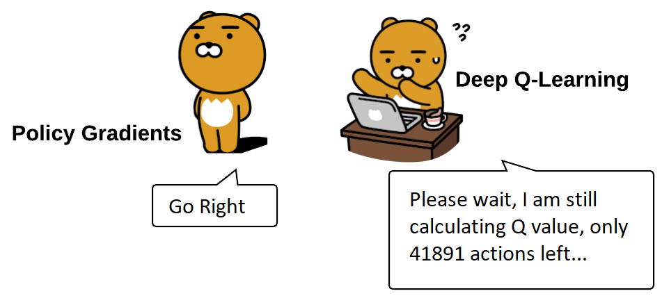
A Note on Sample Inefficiency

Policy gradients require lots of samples. Each batch of rollouts (trajectories) is used once, discarded, and replaced.

Contrast this with Q-learning, where you can replay old games over and over, learning from them repeatedly. This makes policy gradients sample inefficient - you need to play many more games to learn good clicking patterns.

A Note on On-Policy Training

Another challenge you encounter with policy based methods: 

You must train on data collected from the current policy.

If you collect data using an older policy $\pi_{\theta_{t-2}}$, you can’t use it to train $\pi_{\theta_t}$. The mismatch invalidates the gradient estimate.

This is why policy-based methods are called on-policy: learning must track the current behaviour.

Strengths

• Works well in high-dimensional action spaces (like token generation in LLMs)
• Directly optimises the objective (no detour via value functions)
• Stochastic (Randomised) policies = natural exploration

Limitations

• Sample inefficient
• High-variance gradients
• Requires on-policy data
• Struggles with long-term credit assignment (without value estimates)

Wait, Can We Have the Best of Both?

Absolutely! And that's what actor-critic methods aim to do.

Imagine a Minesweeper player who:

1. Has clicking intuition (actor/policy): "I should probably click this tile"
2. Can evaluate board positions (critic/value function): "This board state looks promising for a high score"

By blending both approaches, actor-critic methods harness the strengths of each while mitigating their individual weaknesses.

The critic helps reduce gradient variance by providing better baseline estimates, while the actor maintains the ability to handle complex, high-dimensional action spaces.

This sets the stage for our next chapter: Actor-Critic Methods, where we'll explore how methods like PPO emerged as the go-to choice for training reasoning-capable LLMs.

Stay tuned. We're just getting started!